SWIB
Soil Water Stress, Irrigation Requirement and Water Balance Model
A web-based tool
-
1. About SWIB
SWIB (Soil Water Stress, Irrigation Requirement and Water Balance) is an online model for estimating daily plant/soil water stress (deficit or excess), crop irrigation requirements (and their impact of irrigation on aquifer storage) and water balance components based on measured daily soil moisture and precipitation. SWIB has been developed through a collaborative research effort between Canadian Rivers Institute (CRI), University of New Brunswick (UNB), Agriculture and Agri-Food Canada (AAFC) and Environment and Climate Change Canada (ECCC). SWIB is a result of a larger research effort aimed at evaluating the effects of agricultural production systems on groundwater and surface water quantity and quality. SWIB is part of the Hydrology Tool Set (HTS; https://www.hydrotools.tech), a suite of tools that can be used for advancing the understanding of various local and watershed scale hydrological processes. HTS also includes SepHydro (daily baseflow / hydrograph separation; 11 methods), ETCalc (daily potential, reference and actual evapotranspiration estimation; 8 methods), SNOSWAB (daily estimation of water balance terms, including snowfall, snowmelt, snowpack, soil water content, evapotranspiration, drainage, infiltration, surface runoff), GWRech (daily estimation of groundwater recharge and groundwater discharge), TotPrePart (partitioning of daily total precipitation into snowfall and rainfall) and FLEX-WQI (estimation of water quality state via water quality indexes).
If you used SWIB, please include the following citation(s) in your publication(s):
Danielescu S (2022) SWIB - An Online Model to Estimate Daily Crop Water Stress, Irrigation Needs, and Soil Water Budget. Groundwater.
DOI: https://doi.org/10.1111/gwat.13278.Danielescu S, MacQuarrie K, Zebarth B, Nyiraneza J, Grimmett M, Levesque M (2022) Crop water deficit and supplemental irrigation requirements for potato production in a temperate humid region (Prince Edward Island, Canada). Water 14, 2748.
DOI: https://doi.org/10.3390/w14172748. -
2. Background
The amount of water stored in the soil is the resultant of the interdependence of soil, climate and biota. In addition, management related factors can be an additional driving force for soil water storage for ecosystems that are under significant human impact. For example, for agroecosystems, the irrigation regime can play a significant role on the amount of water stored in the soil during the growing season. Hence, knowledge of the state and dynamics of soil water storage is a key step for advancing our understanding relative to hydrological cycle, ecosystem health or agroecosystem productivity. In particular, soil moisture is a key element for many applications related for example to the impact of severe weather (e.g. droughts) on soil water availability; the impact of water stress (water deficit and excess) on natural vegetation and agricultural crops; the impact of climate change on soil water storage and vegetation; movement of water and solutes (e.g. contaminants) through soil; irrigation requirements for agricultural production; relationship between irrigation water supply and aquifer storage. Other examples of SWIB applications include the evaluation of the significance of soil properties on the dynamics and magnitude of crop water stress (either as water deficit or water excess), impact of irrigation triggering thresholds and scheduling on SWC, effect of irrigation losses on SWC and irrigation water supply requirements, influence of groundwater-sourced irrigation on aquifer storage as well as the evaluation of the various soil water budget components (e.g. evaporative losses, soil moisture losses and gains, soil drainage, infiltration and surface runoff). Broader applications of SWIB include generation of critical data for external models that allow for uploading of user-provided timeseries; or use in educational settings for example to demonstrate the significance of various of concepts related to crop water stress (i.e., water deficit or excess), irrigation practices and soil water balance.
SWIB online model fills an existing gap, by providing unrestricted access to a streamlined and robust framework, which uses a minimal amount of data to estimate daily water deficit and excess, irrigation requirements and impacts of irrigation on aquifer storage as well as several water balance components. SWIB methodology can be applied to any location as long as the required data is provided (e.g. minimal soil properties, daily soil water content and precipitation). Required soil properties (i.e. soil thickness and field capacity) are available either from direct field measurements or alternative sources such as soil surveys and technical guides. Daily soil moisture (i.e. soil water content) data is relatively easy to obtain for example from direct field measurements or from various publicly available databases. Daily precipitation is widely available from various weather monitoring stations. SWIB can be used for testing various scenarios even when field specific critical data (e.g. field capacity) is not available. In addition, the sample data set (i.e. test data) provided allows the user to experiment with the various modules of the model.
SWIB (Soil Water Stress, Irrigation Requirement and Water Balance) integrates three modules: 1) Water Stress (i.e. as water deficit or water excess); 2) Irrigation (and its impact on Aquifer Storage; and 3) Water Balance. The Water Stress module allows for calculation of the number of days with water deficit or water excess as well as of the daily amount of water deficit and/or excess relative to various soil moisture thresholds. The Irrigation module, allows for estimation of the crop irrigation needs, defining an irrigation schedule and calculating the impacts of irrigation on groundwater storage, assuming that groundwater is the main source for the irrigation water. The Water Balance module allows for estimation of several water balance components (e.g. soil water storage gain and loss, infiltration, surface runoff, evapotranspiration above the ground or in the soil) based on soil moisture data provided above and minimal weather data (i.e. precipitation, evapotranspiration). The web-based model provides various output and data visualization options through a streamlined process and a user-friendly interface.
-
3. Methodology
Details regarding data management as well as the methodology used for each of the three modules included in SWIB are presented below.
3.1. Requirements and formatting for input and validation data
Input data is a daily dataset consisting of:
-
Soil moisture (SM). This is a required parameter for the Water Stress, Irrigation and Water Balance modules. SM is required for most of the parameters calculated by the model. SM, represents the Soil Water Content (SWC) and is equal to the soil Volumetric Water Content (VWC). SM is available from in situ measurements or from other sources (e.g. weather stations, online databases, etc.). SM can also be estimated using SNOSWAB (Snow, Soil Water and Water Balance Model; https://snoswab.hydrotools.tech), another tool included in the Hydrology Tool Set (HTS). In the input data file, the units for SM (VWC) are m3/m3;
-
Total precipitation (TP). This is a required parameter for estimating the precipitation deficit (i.e. difference between precipitation and evapotranspiration) in the Irrigation module and the surface runoff in the Water Balance module. TP is the daily total precipitation and includes all forms of precipitation (e.g. snow, rain, freezing rain, etc.). TP is available from in situ measurements or from other sources (e.g. weather stations, online databases, etc.). The units for TP are mm;
-
Evapotranspiration (ET). This is a required parameter for estimating the precipitation deficit (i.e. difference between precipitation and evapotranspiration) and the irrigation water supply in the Irrigation module and evapotranspiration above ground, evapotranspiration in the soil and infiltration the in the Water Balance module. ET is equal to the actual evapotranspiration. Although not directly calculated in SWIB, it can be estimated using ETCALC (https://www.etcalc.hydrotools.tech) or obtained via in situ measurements or other sources (e.g. weather stations, online databases, etc.). The units for ET are mm;
-
Groundwater Recharge (RCH). This is an optional parameter used in the Irrigation module. RCH is equivalent to the net daily groundwater recharge, which is defined as the sum of the daily inflows into the aquifer on the days when the water table elevation of the aquifer is higher than the water table elevation for the previous day. RCH values are used in SWIB for calculating the net impact of irrigation on aquifer storage. RCH can be obtained from various sources (e.g. online databases) or can be estimated using RECHARGE BUDDY, another tool included in the Hydrology Tool Set (https://www.rbuddy.hydrotools.tech), which calculates RCH based on specific yield of the aquifer material and changes in water table elevation. If RCH values are not provided, SWIB will simply calculate the net effect of irrigation on aquifer storage (i.e. SWIB will consider the withdrawal of irrigation water from the aquifer and will ignore the RCH addition of water to aquifer storage). The units for RCH are mm.
Validation data is an optional data subset, and together with Input data forms the user input data file. SWIB allows for up to 5 validation datasets to be included in the user input data file. Validation data provides means for directly comparing any of the data output from SWIB with a dataset obtained using different methods or sources. The validation data set can include evapotranspiration data, soil moisture, soil temperature, groundwater table elevations, etc.
User input data file format: the user input data file has to be uploaded using a file with 1 column dedicated to calendar date, 4 columns dedicated to input data (TP - total precipitation, SM - soil moisture, ETA - actual evapotranspiration, RCH - groundwater recharge) and up to 5 columns dedicated to validation data (VD1 to VD5). The first four columns of the user input data consist of required data (i.e. Date, TP, SM, and ETA) and have to contain values in all rows. The rest of the columns in the user input file (i.e. RCH – groundwater recharge, VD1 to VD5 – validation dataset 1 to 5 are optional and can be left blank. SWIB allows uploading of files with maximum 7500 rows (~20 years of daily data). It is recommended to split the input data set in blocks of 20 years daily timeseries when the intent is to analyze longer time periods.
The number of columns, data format and the units of the various weather parameters required for the input file are shown in the next table:
Columns Date Total Precipitation Soil Water Content Actual Evapotranspiration Groundwater Recharge Validation Data (max 5 columns) Units yyyy-mm-dd mm m3/m3 mm mm user choice Values eg. 2021-12-24 ≥ 0 Between 0 and 1 Between 0 and 200 Between 0 and 500 user choice
Notes:
-
Required data:
Date – use yyyy-mm-dd format;
Total Precipitation [mm];
Soil Water Content [m3/m3]
Actual Evapotranspiration; -
Optional data:
Groundwater recharge [mm];
Validation data [user provided] - leave blank if no data is available -
The model requires daily data
-
Use the first row of the data set for column headings
-
SWIB includes limited input data quality check routines and hence, the user must ensure that the input data set is suitable for analysis (e.g., check dataset for missing values, parameters, erroneous values, etc.)
3.2. Time steps and averaging
SWIB uses daily data for both input and output data. SWIB includes a series of averaging options (i.e. monthly, seasonal [meteorological and growing season], yearly), which are explained in more detail below. Monthly frequency is recommended as the minimum time step for inspecting and analyzing SWIB results. SWIB can also calculate all the output parameters using a “typical year daily” (i.e. daily multi-year averages for each day of the year available in the input file) for the cases when the user input file contains data for more than one year. The monthly as well as the typical daily year (see below for details) are recommended for inspecting and analyzing results when multiple years of data are available. The following time intervals are available in tables, graphs and export files for displaying SWIB results:
-
Daily: this is the operating time step for SWIB;
-
Monthly;
-
Yearly;
-
Meteorological seasons, with the following distribution: Spring: March 1 – May 31st; Summer: June 1st – August 31st; Fall: September 1st – November 30th; Winter: December 1st – February 28th of the following year;
-
Growing season [GS] and outside of growing season [OGS], based on the starting and ending dates specified by the user. OGS spans between the first day after the end of the growing season and the day before the start of the following year’s growing season;
-
Typical year daily: one year of daily data based on the averages of the output data for each day in multiple years (i.e. 365 values) (e.g. for a 5 year daily data set, the value for Jan 1 will be the average for the values on Jan 1 in Year 1,2, 3, 4, and 5). This could be interpreted as the “representative daily year” or “average daily year”;
-
Typical year monthly: one year of monthly averages (i.e. 12 values). The monthly averages are calculated using the typical year daily values;
-
Typical year meteorological season: meteorological season averages (i.e. four values). The meteorological season averages are calculated using the typical year daily values;
-
Typical Year growing season: growing season (GS) and outside of growing season (OGS) averages (i.e. two values). The growing season averages are calculated using the typical year daily values;
-
Yearly: the average for all days in the typical year daily (i.e. one value).
3.3. Additional Parameters and Coefficients Required
-
Input Data Module
Start and end date for the growing season. Used for allowing SWIB to calculate all the parameters for the growing season (GS) and outside of the growing season (OGS). The start and end dates use mm-dd format (the year is ignored as the same dates are applied to all years available in the input data file).
-
Water Stress Module
Layer or Root zone thickness (mm). This is the thickness of the soil layer for which the analyses are conducted. Depending on the analysis it can be interpreted as the thickness of the soil profile, of a horizon or of the root zone. Layer or Root zone thickness is used for converting soil moisture (i.e., Volumetric Water Content) to equivalent height of water column (mm), to allow for calculation of the parameters in the Water Stress, Irrigation and Water Balance modules. The value has to be positive.
Field capacity (m3/m3). Field capacity (FC) is typically equivalent to the water content of the soil at −33 kPa (i.e. −0.33 bar) matric potential. It should be noted that various reference values might be used, for example for sandy soils the -10 kPa (-0.1 bar) pressure is used for determining the field capacity. Field capacity represents the level of the soil moisture 2-3 days after an infiltration event has occurred (e.g. irrigation, snowmelt, rain, etc.), when most of the excess water has already drained from the soil.
Water stress thresholds (T0, T1, T2, T3, T4). (% of FC). These thresholds are used for allowing the estimation of the severity of the water deficit, by calculating the number of days for which the soil is below (T1, T2, T3, T4) or above (T4) certain thresholds. The amount of water deficit or excess (e.g. mm of water) is also calculated for each of these thresholds. The thresholds represent percentages of field capacity (FC) and they can take values between 0 and 100. T0 and T4 are fixed thresholds, with T0 representing zero soil moisture (0% FC) and T4 representing the field capacity (100% FC). T1, T2 and T3 can be adjusted by the user. The percentage value has to increase from T1 to T4. All soil moisture values below T4 are considered to indicate soil water deficit, while soil moisture values above T4 are considered to indicate soil water excess. A scale bar at the bottom of the page shows the position of the various thresholds from a scale ranging from 0 to FC.
-
Irrigation Module
Start and end date of the irrigation period. Allows SWIB to trigger irrigation when SM is below the Irrigation Threshold during the Irrigation period. The format for the start and end dates is mm-dd (the year is ignored as the same dates are applied to all years available in the input data file);
Irrigation threshold (%). During the irrigation period, the soil moisture threshold that triggers supplemental irrigation can be specified. This threshold is expressed as percentage of field capacity, and can have values between 0 and 100. Irrigation starts when soil moisture (SM) drops below this threshold and stops when the threshold is reached;
Irrigation lost to ET (%). This coefficient allows SWIB to estimate the fraction of irrigation water that is lost to evapotranspiration. The irrigation water lost to evapotranspiration is one of the parameters that are included in calculating the irrigation water supply requirement. This coefficient is expressed as percentage of irrigation amount (i.e. irrigation requirement), and hence can have values between 0 and 100. Only the portion of the irrigation water that is left after the application of this coefficient is contributing to increasing soil moisture. This coefficient can also be interpreted as a more comprehensive coefficient for the overall irrigation efficiency, which would account for all the losses from the irrigation system (before the irrigation water enters the soil). As a result of applying this coefficient both the amount of irrigation water and actual evapotranspiration are recalculated. The recalculations impact only the Irrigation module and do not have an impact on the various components calculated with the Water Stress or Water Balance modules;
Irrigation lost to groundwater (%). Allows calculation of the fraction of irrigation water that is returning to groundwater (i.e. return flow). The irrigation water lost to groundwater is one of the parameters that are included in calculating the irrigation water supply requirement. This coefficient is expressed as percentage of irrigation amount (i.e. irrigation requirement), and hence can have values between 0 and 100. As a result of applying this coefficient both the amount of irrigation water and the amount of (net) aquifer storage is recalculated. The recalculations impact only the Irrigation module and do not have an impact on the various components calculated with the Water Balance or Water Stress modules.
-
Water Balance Module
ET Above Soil (%). Allows calculation of the above ground and soil fractions of evapotranspiration. ET Above Soil is expressed as percentage (i.e. %) of evapotranspiration.
3.4. Water Stress Module
Soil water stress, calculated both as water deficit and water excess is based on the daily changes in soil moisture (SM). Based on the difference between soil moisture (i.e. VWC) and field capacity (FC) SWIB calculates if there is water deficit (VWC < FC) or water excess (FC < VWC) in the soil. In addition, several moisture thresholds, as specified by the user, are available for identifying the severity of the water deficit. The number of days with soil moisture below each of the thresholds (i.e. water deficit) as well as above the field capacity (i.e. water excess) and the average difference between these thresholds and VWC are calculated for each day. Independent from soil moisture changes, the precipitation deficit (also known as water deficiency) based on the difference between evapotranspiration (ET) and total precipitation (TP) is also calculated. A positive value indicates precipitation deficit, while a zero value indicates the absence of the precipitation deficit. Precipitation deficit can be used to as an alternative method for assessing crop irrigation requirements, however it does not account for soil moisture or soil properties, hence the soil moisture based method is preferred. The precipitation deficit method is prone to significant errors when calculated on the daily basis and hence, in SWIB this is calculated using on a monthly basis. The monthly averages are distributed to each day in the month in order to obtain a “simulated” daily time series for this type of deficit. However, it should be noted that the water deficit based on soil moisture represents an average (e.g. monthly average), whereas the water deficit based on the difference between precipitation and evapotranspiration is cumulative (e.g. monthly sum), and hence the two parameters are comparable only in terms of trends, but not as absolute quantities. Of note, precipitation deficit can show different dynamics and magnitude when compared with the more accurate, field-based soil moisture deficit method.
3.5. Irrigation Module
The conceptual model used for evaluating the irrigation requirements as well as the impact of irrigation on groundwater recharge is shown in the diagram below. SWIB calculates both the number of days when irrigation is required as well as the irrigation requirement (expressed as mm). The irrigation requirement is defined as the amount of water required to bring soil moisture at user-specified levels (i.e., irrigation thresholds) on days with water deficit (i.e., days with VWC < THR). In SWIB, the portion of irrigation lost to evapotranspiration is calculated based on a user provided coefficient, resulting in both an adjusted ET as well as an adjusted irrigation amount. Similarly, and considering that in SWIB the irrigation water is assumed to be sourced from groundwater, a portion of the irrigation water returns to groundwater (i.e., irrigation return flow). The significance of the return flow is controlled by a user-specified coefficient. The aquifer storage is adjusted following the addition of the return flow to the aquifer.
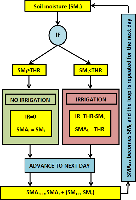
Fig 1. SWIB – Conceptual model for triggering irrigation and adjusting soil moisture based on irrigation schedule
SMt – measured SM on day t; SMt+1 = measured SM on day t+1; THR – SM threshold for triggering irrigation; IR – irrigation requirement; SMAt – adjusted SM on day t; SMAt+1 – adjusted SM on day t+1
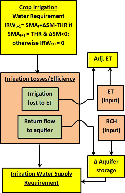
Fig 2. SWIB – Conceptual model for calculating irrigation amounts (crop requirement and water supply) and additional output parameters associated with the Irrigation Module
IRWt+1 –crop Irrigation water requirement on day t+1; ΔSM – change in measured soil moisture between day t and day t+1 (i.e. SMt+1-SMt); SMt+1 = measured SM on day t+1; SMt = measured SM on day t; SMAt+1 - adjusted SM on day t+1; SMAt – adjusted SM on day t; THR – SM threshold for triggering irrigation; ET – evapotranspiration; Adj. ET – ET adjusted using additional ET losses from irrigation; RCH – groundwater recharge; Δ Aquifer storage – adjusted aquifer storage
3.6. Water Balance Module
The conceptual model of SWIB Water Balance module is shown below.
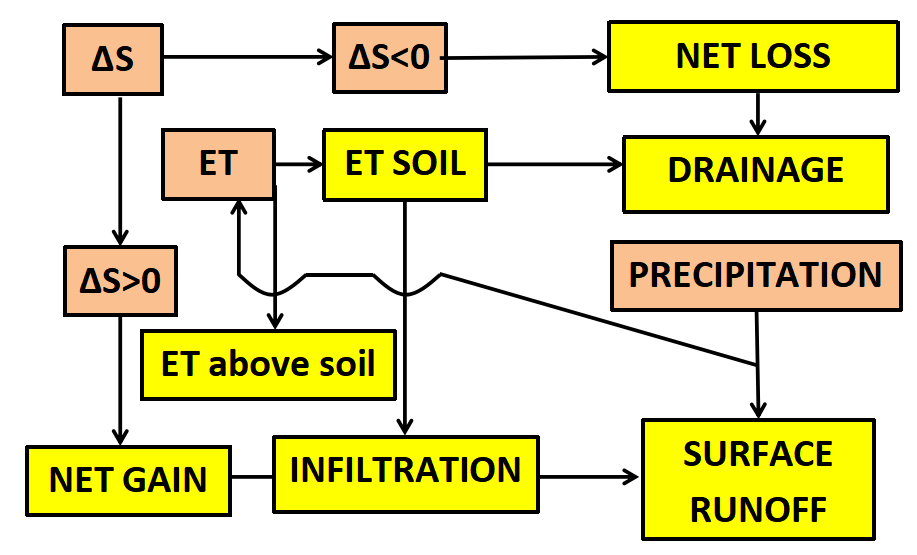
Fig 3. SWIB – Conceptual model for the Water Balance Module
Water balance is calculated using Eqn. 1. Actual evapotranspiration (ET; input data) is divided based on a user provided coefficient into evapotranspiration occurring above the ground due to for example canopy interception, ponding, etc. (ETAS) and evapotranspiration occurring in soil (ETFS). The daily soil moisture loss (i.e., Net loss) is calculated as the difference in measured soil water content between two consecutive days, when this difference is negative. The Net loss values for various averaging intervals is obtained by adding the daily net losses. Daily drainage (DR) is calculated as the difference between Net loss and the fraction of evapotranspiration occurring in the soil (ETFS), when this difference is positive and is considered to be absent when this difference is zero or negative. Soil is considered to gain moisture (i.e. Net gain) when the difference in measured soil water content between two consecutive days is positive. Infiltration and surface runoff can occur only on the days with Net gain in soil water storage. Infiltration (INF) is equal to the sum of daily Net gain and the fraction of evapotranspiration occurring in the soil profile. Surface runoff (SR) is calculated based on the difference between precipitation and infiltration. However, daily SR calculations could be subject to errors due to the delay between the time of precipitation and the actual response in soil moisture, as well as due to the possible presence of snowfall, snowpack and snowmelt during the colder periods of the year. Thus, the calculation of SR is based by default on a four-day window, with SR calculation triggered only for the windows when the average soil moisture content in the last two days of the window is larger than the average soil moisture content in the first two days of the same window (i.e. indicating that an infiltration event has occurred). The width of the window (i.e. number of days) for the calculation of surface runoff can be modified by the user. OTH represents losses or gains that are not accounted for and can also be interpreted as the budget error. OTH can be the result of the various assumptions used by the model as well as rounding up errors, and can be expressed as absolute value (mm; Eqn.1) or as percentage of total inputs (Eqn. 2).

Eq 1. - Total Precipitation
TP - Total Precipitation (mm)
ETAS - Evapotranspiration above Soil (mm)
ETFS - Evapotranspiration from Soil
ΔS - change in soil water storage (mm) [SWC Net Gains - SWC Net Losses]
DR - Drainage (mm)
SR - Surface Runoff (mm)
SWC - Soil Water Content (mm)
OTH - unaccounted losses or gains (mm) [budget error]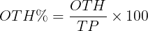
Eq 2. - Unaccounted losses or gains
OTH % - Unaccounted losses or gains (%) [budget error]
All the calculations for the water balance are performed using millimetres of water (mm) units. Soil moisture (i.e. volumetric water content; VWC), which has units of m3/m3 in the user input file is converted to millimetres using the thickness of the soil specified by the user. The rates for the various water balance components (e.g., infiltration rate, drainage rate, etc.) can be calculated by dividing the values for the various components to the extent of the averaging interval.
3.7. Output Parameters
Below is a list off all coefficients and output parameters available in SWIB. These parameters are available via Table View and Export Data menu tabs.
Water Stress Module
- SWC in Soil (mm): measured soil moisture
- Def. SWC < T1 (m3/m3 or mm): amount of soil moisture below T1 (soil water deficit)
- Def. SWC < T2 (m3/m3 or mm): amount of soil moisture below T2 (soil water deficit)
- Def. SWC < T3 (m3/m3 or mm): amount of soil moisture below T3 (soil water deficit)
- Def. SWC < FC (m3/m3 or mm): amount of soil moisture below FC (soil water deficit)
- Exc. SWC > FC (m3/m3 or mm): amount of soil moisture above FC (soil water excess)
- Def. SWC < T1 (days): day with soil moisture below T1 (soil water deficit)
- Def. SWC < T2 (days): day with soil moisture below T2 (soil water deficit)
- Def. SWC < T3 (days): day with soil moisture below T3 (soil water deficit)
- Def. SWC < FC (days): day with soil moisture below FC (soil water deficit)
- Exc. SWC > FC (days): day with soil moisture above FC (soil water excess)
- Def. ET-PP (mm): amount of precipitation deficit (>0 indicates precipitation deficit)
Irrigation Module
- In Irrig. Season (days): Days during or outside of the irrigation season
- SWC in Soil (mm): measured soil moisture
- Change in SWC (mm): change in measured soil moisture between consecutive days
- Irrig. Required (days): irrigation required to increase soil moisture to irrigation threshold (i.e. to stop irrigation)
- SWC after Irrig. (mm): soil moisture after irrigation
- Irrig. Water Added (mm): amount of irrigation water added
- Water Supply Req. (mm): amount of irrigation water supply, including losses to evapotranspiration and return flow to aquifer
- GW Rech. (mm): groundwater recharge (optional input data)
- Change in Aquifer Storage (mm): net impact of irrigation water supply on aquifer storage. Accounts for groundwater recharge (if provided) and irrigation water supply (i.e. does not consider return flow; >0 indicates that the aquifer is gaining water; < 0 indicates that the aquifer is losing water)
- Irrig. Ret. Flow (mm): fraction of irrigation water that is returning to the aquifer (>0 indicates return flow)
- Change in Aquifer Storage Adj. (mm): net impact of irrigation water supply on aquifer storage. Accounts for groundwater recharge (if provided), irrigation water supply and return flow (>0 indicates that the aquifer is gaining water; < 0 indicates that the aquifer is losing water)
- ET Adj. (mm): evapotranspiration adjusted with losses of irrigation water to evapotranspiration
- Def. ET-PP (mm): amount of precipitation deficit (>0 indicates precipitation deficit)
Water Balance Module
- SWC in Soil (mm): measured soil moisture
- Precip. (mm): total precipitation (includes all forms of precipitation)
- ET Total (mm): total (actual) evapotranspiration
- ET above Ground (mm): fraction of evapotranspiration occurring above ground (e.g. canopy interception, ponding, etc.)
- ET from Soil (mm): fraction of evapotranspiration occurring in the soil
- Net Loss (mm): net water loss from the soil layer
- Net Gain (mm): net water gain by the soil layer
- Drainage (mm): amount of water draining from the soil layer
- Infiltr. (mm): amount of water infiltrating into the soil layer
- Surf. Runoff (mm): amount of surface runoff
Metadata
- GS_start_day: first day of the growing season
- GS_start_month: starting month of the growing season
- GS_end_day: last day of the growing season
- GS_end_month: ending month of the growing season
- Layer or Root zone thickness (mm): thickness of the (soil) layer for all calculations
- Field capacity (m3/m3): field capacity of the soil layer
- SWC T1 deficit threshold (%FC or m3/m3): T1 threshold for calculating soil water deficit
- SWC T2 deficit threshold (%FC or m3/m3): T2 threshold for calculating soil water deficit
- SWC T3 deficit threshold (%FC or m3/m3): T3 threshold for calculating soil water deficit
- Irrigation_start_day: first day of the irrigation period
- Irrigation_start_month: starting month of the irrigation period
- Irrigation_end_day: last day of the irrigation period
- Irrigation_end_month: ending month of the irrigation period
- Irrigation_trigger_threshold (%FC or mm): soil moisture threshold for triggering irrigation
- Irrigation_lost_to_ET (%): coefficient for calculating the fraction of irrigation water lost to evapotranspiration
- Irrigation_lost_to_GW (%F): coefficient for calculating the fraction of irrigation water lost to groundwater (i.e. return flow)
- ET_loss_above_soil (%): coefficient for calculating the fraction of evapotranspiration occurring above ground
Statistics
- Average: average of the parameter (full dataset)
- Minimum: minimum of the parameter (full dataset)
- Maximum: maximum value of the parameter (full dataset)
- Std Dev: standard deviation of the parameter (full dataset)
-
-
4. User Guide
SWIB is a web based model that allows calculation of soil water stress (i.e. soil water deficit and soil water excess), crop irrigation and irrigation water supply requirements, the impact of irrigation on aquifer storage as well as various (soil) water balance components on a daily basis. The model provides tabular and graphical representations of the input data, output data, and validation data, as well as representative statistics for various time intervals including daily, monthly, meteorological and growing seasons, yearly and various averaging intervals for multiyear data sets (see section 3.2. Time steps and averaging).
At the top, a contextual menu provides access to the various modules of the tool. The modules can be accessed progressively, in the following order: 1) Home (Information module); 2) Input Data (Data entry module); 3) Water Stress (Calculation module); 4) Irrigation (Calculation module); and 5) Water Balance (Calculation module). Once a calculation module has been completed the user is able to return to the respective module at any time during the session. A set of additional menu tabs is available for the data entry (i.e., Info, Load Data, Table View, Graphical View and Export Data) and calculation (i.e., Info, Analysis, Table View, Graphical View and Export Data) modules. In the following sections the options available under the Input Data – Load and under the Analysis menu tab of each calculation module will be presented in separate subsections. The options available under the other menu tabs are presented as a separate subsection.
4.1. Quick start
In order to run SWIB the user has to go through the following steps:
-
Load Data: provide required data or use the provided test data [Input Data module];
-
Perform Water Stress calculations: enter required parameters and select Run Water Stress Analysis [Water Stress module – Analysis];
-
Perform Irrigation module calculations: enter required parameters and select Run Irrigation Analysis [Irrigation module – Analysis];
-
Perform Water Balance calculations: enter required parameters and select Run Water Balance Analysis [Water Balance module – Analysis];
-
Investigate Results and Export Data: Review SWIB output from each module [Table View and/or Graphical View] and export results [Export Data menu or CSV button under each data entry and calculation modules].
The steps required for using the model are described in more detail below.
4.2. Home Module
This module contains information related to the development, methodology and use of SWIB. Under each of the input and calculation modules an Info tab is available, where general information relevant to the respective module is provided.
4.3. Load Data (Input Data Module)
The first step in conducting an analysis is to upload the input data file to be used in SWIB. The users can run SWIB either by using the test dataset or by uploading a new dataset.
For practicing with SWIB and better understanding how the various components of the model work, the user can use the test data set provided (two years of daily data), by clicking on “Try the tool using the test dataset” button. The test dataset contains two years of daily required data and validation data for a research site located at the Agriculture and Agri-Food Canada (AAFC) Harrington Experimental Farm (Charlottetown, Prince Edward Island). The validation data included in the test dataset consists of daily water table elevations (VD1) and air temperature (VD2).
For using SWIB the users can upload their own datasets. The model accepts source data sets in Comma Separated File (csv) format. The users can use the “Download Sample File” button located on the Upload User Data Page (Load Data) or the “Export Input Data - Daily” menu to obtain a correctly formatted input file that can be used as a model for populating the input data file with user data. The user input file can be uploaded to SWIB by using the “Upload user data” button. SWIB allows uploading of files with maximum 7500 rows (~20 years of daily data). It is recommended to split the input data set in blocks of 20 years daily timeseries when the intent is to analyze longer time periods. It should be noted that the model cannot accommodate missing data (i.e. blank rows in required data columns) or erroneous data entries, and hence it is recommended that the integrity of the source data is verified before uploading. An error message will be displayed, and the user will be redirected to the Load Data page if inconsistencies are detected in the user file.
The input data file consists of a tabular file with 1 column dedicated to calendar date, 4 columns dedicated to input data (TP - total precipitation, SM - soil moisture, ETA - actual evapotranspiration, RCH - groundwater recharge) and up to 5 columns dedicated to validation data (VD1 to VD5). The first four columns of the user input data consist of required data (i.e. Date, TP, SM, and ETA) and have to contain values in all rows. The rest of the columns in the user input file (i.e. RCH – groundwater recharge, VD1 to VD5 – validation dataset 1 to 5) are optional and can be left blank if data is not available. The validation data sets are not restricted to certain parameters and can include time series for any parameter that the user would like to use for comparing with the output from SWIB. Examples of validation datasets include drainage, evapotranspiration, soil moisture, soil temperature, groundwater table elevations, etc.
The number of columns, data format and the units of the various weather parameters required for the input file are shown in the next table:
Columns Date Total Precipitation Soil Water Content Actual Evapotranspiration Groundwater Recharge Validation Data (max 5 columns) Units yyyy-mm-dd mm m3/m3 mm mm user choice Values eg. 2021-12-24 ≥ 0 Between 0 and 1 Between 0 and 200 Between 0 and 500 user choice Notes:
-
Consult section 3.1. Requirements and formatting for input and validation data for a detailed explanation of all the parameters used in the input data file
-
Required data:
Date – use yyyy-mm-dd format;
Total Precipitation [mm];
Soil Water Content [m3/m3]
Actual Evapotranspiration; -
Optional data:
Groundwater recharge [mm];
Validation data [user provided] - leave blank if no data is available -
The model requires daily data
-
Use the first row of the data set for column headings
-
SWIB includes limited input data quality check routines and hence, the user must ensure that the input data set is suitable for analysis (e.g., check dataset for missing values, parameters, erroneous values, etc.)
On this page the user can specify the beginning and the end of the growing season in the boxes provided at the bottom of the page. These dates are used for averaging the various parameters during the growing season (GS) and outside of the growing season (OGS). In SWIB, it is assumed that these dates are not changing from year to year and hence, the start and end dates use the mm-dd format (the year is ignored as the same dates are applied to all years available in the input data file).
Once the input dataset is loaded to SWIB via the Load Data button, the view switches to Table View. See section 4.7. for instructions regarding the inspection of datasets using tables and graphs as well as for the various options available for exporting the data.
Once the loading and inspecting of the input data is completed the user can click on the Water Stress menu entry at the top of the page to advance to the first calculation module.
Consult section 3.1. and section 3.3. for more details.
4.4. Analysis - Water Stress Module
On the Analysis Tab the user has to provide:
-
Layer or Root zone thickness (mm). This is the thickness of the soil layer for which the analyses are conducted. Depending on the analysis it can be interpreted as the thickness of the soil profile, of a horizon or of the root zone. Layer or Root zone thickness is used for converting soil moisture (i.e., Volumetric Water Content) to equivalent height of water column (mm), to allow for calculation of the parameters in the Water Stress, Irrigation and Water Balance modules. The value has to be positive;
-
Field capacity (m3/m3). Field capacity (FC) is typically equivalent to the water content of the soil at −33 kPa (i.e. −0.33 bar) matric potential. It should be noted that various reference values might be used, for example for sandy soils the -10 kPa (-0.1 bar) pressure is used for determining the field capacity. Field capacity represents the level of the soil moisture 2-3 days after an infiltration event has occurred (e.g. irrigation, snowmelt, rain, etc.), when most of the excess water has already drained from the soil;
-
Water stress thresholds (T0, T1, T2, T3, T4). (% of FC). These thresholds are used for allowing the estimation of the severity of the water deficit, by calculating the number of days for which the soil is below (T1, T2, T3, T4) or above (T4) certain thresholds. The amount of water deficit or excess (e.g. mm of water) is also calculated for each of these thresholds. The thresholds represent percentages of field capacity (FC) and they can take values between 0 and 100. T0 and T4 are fixed thresholds, with T0 representing zero soil moisture (0% FC) and T4 representing the field capacity (100% FC). T1, T2 and T3 can be adjusted by the user. The percentage value has to increase from T1 to T4. All soil moisture values below T4 are considered to indicate soil water deficit, while soil moisture values above T4 are considered to indicate soil water excess. A scale bar at the bottom of the page shows the position of the various thresholds from a scale ranging from 0 to FC.
Once the parameters are set the user can click on the Run Water Stress Analysis button and the view will switch to Table View. See section 4.7. for instructions regarding the inspection of datasets using tables and graphs as well as for the various options available for exporting the data.
The user can click on the Irrigation menu entry at the top of the page to advance to the next calculation module.
Consult section 3.3. and section 3.4. for more details.
4.5. Analysis - Irrigation Module
On the Analysis Tab the user has to provide:
-
Start and end date of the irrigation period. Allows SWIB to trigger irrigation when SM is below the Irrigation Threshold during the Irrigation period. The format for the start and end dates is mm-dd (the year is ignored as the same dates are applied to all years available in the input data file);
-
Irrigation threshold (%). During the irrigation period, the soil moisture threshold that triggers supplemental irrigation can be specified. This threshold is expressed as percentage of field capacity, and can have values between 0 and 100. Irrigation starts when soil moisture (SM) drops below this threshold and stops when the threshold is reached;
-
Field capacity (FC). This field is simply displaying the field capacity as entered in the Water Stress module (%, mm). The value can be changed in the Analysis – Water Stress module and the Water Stress Analysis has to be re-run for the change to be carried over into the Irrigation module.
-
Irrigation lost to ET (%). This coefficient allows SWIB to estimate the fraction of irrigation water that is lost to evapotranspiration. The irrigation water lost to evapotranspiration is one of the parameters that are included in calculating the irrigation water supply requirement. This coefficient is expressed as percentage of irrigation amount (i.e. irrigation requirement), and hence can have values between 0 and 100. Only the portion of the irrigation water that is left after the application of this coefficient is contributing to increasing soil moisture. This coefficient can also be interpreted as a more comprehensive coefficient for the overall irrigation efficiency, which would account for all the losses from the irrigation system (before the irrigation water enters the soil). As a result of applying this coefficient both the amount of irrigation water and actual evapotranspiration are recalculated. The recalculations impact only the Irrigation module and do not have an impact on the various components calculated with the Water Stress or Water Balance modules;
-
Irrigation lost to groundwater (%). Allows calculation of the fraction of irrigation water that is returning to groundwater (i.e. return flow). The irrigation water lost to groundwater is one of the parameters that are included in calculating the irrigation water supply requirement. This coefficient is expressed as percentage of irrigation amount (i.e. irrigation requirement), and hence can have values between 0 and 100. As a result of applying this coefficient both the amount of irrigation water and the amount of (net) aquifer storage is recalculated. The recalculations impact only the Irrigation module and do not have an impact on the various components calculated with the Water Balance or Water Stress modules.
Once the parameters are set the user can click on the Run Irrigation Analysis button and the view will switch to Table View. See section 4.7. for instructions regarding the inspection of datasets using tables and graphs as well as for the various options available for exporting the data.
The user can click on the Water Balance menu entry at the top of the page to advance to the next calculation module.
Consult section 3.1. and section 3.5. for more details.
4.6. Analysis - Water Balance Module
On the Analysis Tab the user has to provide:
-
Layer or Root zone thickness (mm). This field is simply displaying the thickness of the layer as entered in the Water Stress module (mm). The value can be changed in the Analysis – Water Stress module. If this value is changed the Water Stress Analysis has to be re-run for the change to be carried over into the Water Balance module;
-
ET Above Soil (%). Allows calculation of the above ground and soil fractions of evapotranspiration. This parameter can have values between 0 and 100.
-
Window width for SR calculation (days). The value in this field sets the width of the window for surface runoff calculation. The minimum value is 2 (days).
Once the parameters are set the user can click on the Run Water Balance Analysis button and the view will switch to Table View. See section 4.7. for instructions regarding the inspection of datasets using tables and graphs as well as for the various options available for exporting the data.
The user can click on any of the menu entries at the top of the page to access the various modules available.
Consult section 3.3. and section 3.6. for more details.
4.7. Data inspection, visualisation and export (all modules)
Inspection of data via tabular and graphical views can be conducted via the Table View, Graphical View and Export Data menu entries that become available in the Input Data module once the input dataset is loaded to SWIB. These menu entries are also available under each of the calculation modules (Water Stress, Irrigation and Water Balance), and allow the user to evaluate the output for each of these modules.
Table View allows the user to display data in tabular format using various time steps and intervals (see Section 3.2. Time steps and averaging for more details). The user can also change the number of lines, filter data based on date or adjust the starting date of the data that is displayed. For the Water Stress module, the user is provided with the option of changing the measurements units of the values displayed in the table (i.e. m3/m3, mm, %). In addition, in the Water Stress Module, the user can switch between displaying the amount of water deficit/excess for each soil moisture threshold and displaying the corresponding number of days for each threshold. Statistics for the entire dataset are shown below the main table. The tables shown on this page, including either data lines or statistics can be exported individually by using the CSV button located to the right of each of the tables (i.e. only the data shown in the current window will be exported).
Graphical View allows for plotting of input or output data using various time steps and intervals (see Section 3.2. Time steps and averaging for more details) available via a drop-down menu. The parameters that can be displayed are available in the selection pane located to the right of the plot. Each parameter can be displayed on the primary (left) Y axis or on the secondary (right) Y axis by clicking on the toggle placed at the right of the selection pane. Additional options for adjusting the plot become visible when the mouse pointer is placed above the plot. These options include zoom, auto scale, reset axes, show data point labels, export plot, etc. Statistics the entire dataset are shown below the plot. The statistics table displayed below the graph can be exported individually by using the corresponding CSV button located to the right of the page.
The Export Data tab offers additional options for exporting the entire dataset using various time steps and intervals (see Section 3.2. Time steps and averaging for more details). The Export Data Tab also provides options for exporting statistics and metadata (i.e. parameters and coefficients used by the user in the respective module) The data is currently exported in csv format. The csv button located at the top right of each table in Table View or in Graphical View can be used if the intent is to export only the data shown in the current window.
Consult section 3.2. and section 3.7. for more details.
-
-
5. Limitations
SWIB allows uploading of files with maximum 7500 rows (~20 years of daily data). It is recommended to split the input data set in blocks of 20 years daily timeseries when the intent is to analyze longer time periods.
SWIB includes limited input data quality check routines. Hence, the user is advised to conduct a thorough data quality check before uploading input data to minimize the risk for erroneous output.
Daily surface runoff calculations could be subject to errors due to the delay between the time of precipitation and the actual response in soil moisture (1-2 days) as well as due to the possible presence of snowfall, snowpack and snowmelt during the colder periods of the year.
-
6. Terms of Use
SWIB can be used freely.
The authors do not assume any responsibility for the model's operation, output, interpretation, or use of results.
-
7. Contact
Serban Danielescu, Ph.D.
Research Scientist | Chercheur scientifique
Environment and Climate Change Canada | Environnement et Changements Climatiques Canada
Agriculture and Agri-Food Canada | Agriculture et Agroalimentaire Canada
Fredericton Research and Development Centre | Centre de recherche et développement de Fredericton
95 Innovation Rd., Fredericton, NB, E3B 4Z7
Telephone/Téléphone: 506-460-4468
Facsimile/Télécopieur: 506-460-4377
